Developing Real-Time Evolving Deep Learning Model of Hydro-Plant Operations
By William Girard
INTRODUCTION
The United Nations’ (UN’s) recent reports have heralded to the world that there is a pressing need to secure a livable and sustainable future for all, as the window of opportunity is rapidly closing [1]. UN Secretary-General Antonio Guterres estimates renewables must double to 60 percent of global electricity by 2030 for us to be on track [1]. Climate change has undoubtedly become the premiere issue of the 21st century, and this research sought to integrate recent advances in deep learning [2] to conduct disruptive research in this field. Our area of interest was in the renewable sector, specifically hydropower plants. Hydropower, as the largest source of renewable electricity, [3] is critical in slowing down the rising temperatures; however, many of the current hydropower plants need modernization [3].
The IRENA report reveals that the average age of hydropower plants is close to 40 years old and highlights that aging fleets pose a real challenge in several countries. Fig. 1 illustrates how plants in North America and Europe, in particular, are significantly aged.
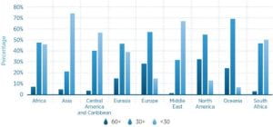 |
| Fig. 1 – Age of Hydropower Plants by Region |
The badly needed upcoming renovations of hydro-plants provide an excellent opportunity to integrate real-time evolving models, a type of machine learning model that improves its accuracy with real-time data [4], into day-to-day plant operations. This real-time model would be able to accurately predict the upcoming energy output of the plant, allowing plant managers to run the hydro-plant with increased efficiency. Currently, this form of deep learning aided decision making is not present in hydro-plants. Bernardes et al. identified real-time schedule forecasting as a new area for disruptive research, showcasing the potential for real-time research [5]. Based on descriptions in job listings, plant operators focus on maintaining equipment and safe plant operations [6]. Assisted by a deep learning model, the plant operators could make better educated decisions based on the model output. These decisions could include the speed of the turbines, the number of turbines running, or how much energy to save in reserve. This paper will be introducing a real-time artificial neural network, and a traditional artificial neural network, and will compare the effectiveness of each approach. Since the model will be predicting a singular energy value, this is a regression problem [7]. Both techniques will be using the popular backpropagation method, which utilizes a stochastic gradient descent optimizer to fine tune each neuron based on the error of the predicted values [8]. As such, the first neural network will be a backpropagation neural network (BPNN) and then the real-time backpropagation neural network (RT-BPNN) will be introduced.
The standard BPNN approach will be implemented using the concept of an input layer, hidden layers, and an output layer. The neurons will be activated using activation functions and the results of the ANN are expected to be rather average for a real-time implementation. The traditional BPNN will be trained on a subsection of the data, and then incrementally tested on the remaining points. The RT-BPNN will be trained incrementally, and then tested on upcoming data points as the model progresses. This paper seeks to prove the incremental approach greatly improves on the traditional BPNN and has above satisfactory results, especially for daily datapoints.
DATASET CREATION
The limited selection of hydropower energy generation datasets necessitated the creation of a suitable dataset from scratch. The first step to achieving a suitable dataset for energy prediction is finding a dataset with energy outputs of various hydropower plants. The data must be suitable for a real-time environment, therefore daily energy outputs were preferable. However, since this paper is a proof of concept, simulated data points would be deemed acceptable. The simulated points would be from monthly data points at worst, since simulated data points from a yearly average would be far too inaccurate. Table 1 lists the chosen input parameters and energy, including name, units, and a short description:
Table I. Input Parameters
| Parameter Name |
Units |
Short Description |
| Day |
Unitless |
Days numbered 1-365 or 1-366 on leap year |
| Temperature |
Fahrenheit |
Average daily temperature |
| Temperature Departure |
Fahrenheit |
Temperature departure from historical mean |
| Heating Days |
Unitless |
Number illustrating expected energy used to heat a house |
| Cooling Days |
Unitless |
Number illustrating expected energy used to cool a house |
| Precipitation |
Inches |
Daily recorded rainfall |
| Stream Flow |
Cubic feet per second |
Cubic feet per second of the river attached to the dam |
| Net Energy |
Megawatt-hour |
Daily energy output of the plant |
Most of the input parameters in Table 1 were chosen from Zhou et al., who outlined relevant factors affecting hydropower generation [9]. The input parameters help model the streamflow and the weather, two major factors affecting hydropower generation. The heating days and cooling days input parameters are slightly more complicated. The degree days assume that a temperature of 65 degrees Fahrenheit means no heating or cooling is required to be comfortable. If the temperature mean is above 65°F, you subtract 65 from the mean and the result is Cooling Degree Days. If the temperature mean is below 65°F, we subtract the mean from 65 and the result is Heating Degree Days [10]. A monthly energy dataset was found named RectifHyd. This dataset provides estimated monthly hydroelectric power generation for approximately 1,500 plants in the United States [11]. Two hydropower plants were chosen, the Black Canyon Dam in Indiana and the Flaming Gorge Dam in Utah. A year range of six was chosen, from 2015 to 2020. The monthly datapoints were first simulated into daily datapoints using the calendar, random, and csv Python libraries. The nearest river to the Black Canyon Dam is Payette River and the nearest river to the Flaming Gorge Dam is Green River. The United States Geological Survey (USGS) provides a free service named Surface-Water Historical Instantaneous Data for the Nation [12]. The streamflow data was extracted and then added to the appropriate test datasets. The National Weather Service provides a service named NOWData [13]. After choosing a weather station, a table is outputted with daily data for a month. Temperature, precipitation, temperature departure, cooling days, and heating days were all gathered from this resource. The data is already available as daily data entries, so no further processing is needed.
TRADITIONAL APPROACH
The traditional approach involves using TensorFlow’s Keras to build a sequential model. Keras is the high-level API for TensorFlow and contains straight forward functions for deep learning. More information about Keras can be found in the documentation on TensorFlow’s website [14]. A sequential model is a plan stack of layers where each layer has only one input tensor and output tensor. Therefore, the sequential model cannot be used for implementations that require multiple inputs and outputs or if you require a non-linear model [15]. The Keras model contains an input layer, hidden layers, and an output layer. The input layer is created by using one neuron for each input parameter. The Dense function is then to create three hidden layers. Each hidden layer is a collection of densely packed neurons that connect to the next hidden layer or output layer. Every layer has their own associated weight and bias in addition to an activation function [16]. The output layer is then created with a singular neuron since this is a regression problem. The model is compiled with the popular loss function of Mean Squared Error (MSE) and Mean Absolute Error (MAE) as an additional metric. The model is then trained using the fit function with a set number of iterations, commonly known as epochs, a proper batch size, and a validation split. This implementation used the popular 20% validation split. Table 2 shows the chosen tuning parameters and the testing methodology.
Table II. Tuning Hyperparameters
| Parameter name |
Chosen value |
Min value |
Max value |
Methodology |
| Activation Function |
ReLu |
N/A |
N/A |
Tested activation functions: ReLu, Leaky ReLu, and Swish |
| Neurons Layer 1 |
128 |
4 |
512 |
Increment neurons by powers of 2 |
| Neurons Layer 2 |
64 |
4 |
512 |
Increment neurons by powers of 2 |
| Neurons Layer 3 |
32 |
4 |
512 |
Increment neurons by powers of 2 |
| Learning Rate |
0.004 |
0.0001 |
0.1 |
Decrement by 0.03, 0.003, or 0.0003 each time |
| Epochs |
500 |
N/A |
N/A |
Used early stopping and graph modeling to determine value |
| Batch size |
32 |
2 |
128 |
Increment by powers of 2 |
Once the tuning parameters were finished being chosen, the model would then be evaluated. To accurately compare results with the incremental approach, the model was tested incrementally. The optimal batch size for the real-time implementation was chosen to be 30. Therefore, the traditional approach would be tested on the first day of each month, the first week of each month, and the entire month. Once the MAE is collected, the model training and evaluation is complete.
 |
| Fig. 2 – Loss and MAE Graph – Dataset 1 Improved |
 |
| Fig. 3 – Loss and MAE Graph – Dataset 2 Improved |
Subsequent tests concluded the model was overfitting, in other words, the validation loss was higher than the training loss. This was solved by dropping out 40% of the neurons for the first test dataset and 20% of the neurons for the second test dataset. The average accuracies without Dropout were: 76% daily accuracy, 82.1% weekly accuracy, and 80% monthly accuracy. The average accuracies with dropout were: 80% daily accuracy, 86% weekly accuracy, and 84% monthly accuracy. The second test dataset saw the average accuracies go from ~69% across the board to ~80%. Figure 2 shows the improved graph for the first test dataset and Figure 3 shows the improved graph for the second test dataset. The execution time of the program is respectable. It can complete 500 iterations in under a minute on a computer with a 2.6 GHz processor and 16 GB of RAM.
ANN REAL-TIME APPROACH
The architectural design of the real-time model can be visualized by Figure 4.
 |
| Fig. 4 A flowchart of the real-time approach |
The first major step is the initialization of the model on historical plant data. The initialization of the model is necessary for reasonable model accuracy. Without the initialization set, the model adapts to the data too slowly for real-time implementation. For this approach, the model will be initialized on the first year of data and the remaining five years will be used in the main training loop. The initialization is conducted using the standard Sequential model discussed in the previous section. The initialization is completed in around 15 seconds, a reasonable amount of time.
The approach to the real time training loop is that of an incremental model. In the incremental approach, the entire dataset is not available to the model so the points are instead fed incrementally as time passes. The model must then adapt to this data, hence the name ‘evolving’ or ‘incremental’ model. Our approach simulates this real-time environment by feeding the data into the model in batches and employing the window strategy outlined in Figure 5 and used in Ford et al. [17].
 |
| Fig. 5 A flowchart of the window approach |
The optimal data points per batch was chosen to be thirty. The model is trained on the 30 data points using Keras’ train_on_batch method a set number of epochs. The batch of 30 is then removed and a new batch of 30 is added. To simulate the model’s performance in a real-time environment, the model is evaluated on the next day outside of the training window, the next week outside of the training window, and the next month outside of the training window.
REAL TIME MODEL RESULTS ANALYSIS
Once the real-time model was compiled, testing of the tuning parameters must begin. Unlike the other tuning parameters, the optimizer and activation function were tested using GridSearchCV from the sklearn library. The optimal optimizer and activation function were found to be RMSprop [18] and Leaky ReLU [19] respectively. The remaining tuning parameters were tested manually, and the results are shown in Table 3.
Table III. Manual Testing of Tuning Parameters
| Parameter name |
Chosen value |
Min value |
Max value |
Methodology |
| Neurons Layer 1 – Test Dataset 1 |
1028 |
4 |
1028 |
Increment neurons by powers of 2 |
| Neurons Layer 2 – Test Dataset 1 |
16 |
4 |
1028 |
Increment neurons by powers of 2 |
| Neurons Layer 3 – Test Dataset 1 |
4 |
4 |
1028 |
Increment neurons by powers of 2 |
| Neurons Layer 1 – Test Dataset 2 |
1028 |
4 |
1028 |
Increment neurons by powers of 2 |
| Neurons Layer 2 – Test Dataset 2 |
256 |
4 |
1028 |
Increment neurons by powers of 2 |
| Neurons Layer 2 – Test Dataset 2 |
8 |
4 |
1028 |
Increment neurons by powers of 2 |
| Learning Rate |
0.003 |
0.0005 |
0.1 |
Decrement each time |
| Epochs |
35 |
5 |
50 |
Increment by 5 each test |
| Window speed |
30 |
7 |
30 |
Test one week, two weeks, one month |
| Window size |
30 |
7 |
90 |
Test one, two, or three times the window speed |
These are the average accuracies of the first dataset over ten tests: daily: 90.26%, weekly: 88.6%, and monthly: 79.6%. These are the average accuracies of the second dataset over ten tests: daily: 92.54%, weekly: 89.31%, and monthly: 83.61%. Compared to the traditional BPNN, the first dataset had its accuracy improved by 10% for daily points, 2.6% for weekly points, and the monthly accuracy decreased by 4%. The second dataset had its accuracy improved by 12.5% for daily, 9.3% for weekly, and 3.6% for monthly. Although the monthly accuracy barely changing or decreasing may seem surprising, the major benefit of the incremental approach is an increase in accuracy for real-time application. The greatly improved daily accuracy, 10% and 12.5%, shows the large benefit of the incremental approach for predicting singular points close to the training window.
Useful graphs can be created to analyze the accuracy of the model. Figure 6 shows the
 |
| Fig. 6 Daily, Weekly, and Monthly plot for test dataset one |
 |
| Fig. 7 Daily, Weekly, and Monthly plot for test dataset two |
graph for the first test dataset and Figure 7 shows the graph for the second test dataset. For both graphs, the daily accuracy has a low number of downward spikes, indicating the model has sufficiently learned from the training. Since the model is trained on thirty datapoints at a time, it captures day-to-day trends very well, resulting in consistent and impressive daily energy predictions. The weekly accuracy is also consistent, although it does experience a few downward accuracy spikes. This is likely because the model has more difficulty predicting points further away from its training window. The monthly accuracy, unsurprisingly, is the most variable. The points furthest away from the training window will be difficult to predict, resulting in lower accuracy. Additionally, extreme weather can drop model accuracy. Examples include a hurricane, a very rainy day, or a flood. A further research path would be implementing a weather forecasting model to assist the central model with more accurate energy forecasting.
The model can complete a full training cycle, including evaluation, in around half a second on a system with a 2.8 GHz processor with 16 Gigabytes of installed RAM. The time per batch is also very constant. Please note that processing times would be even faster on a GPU with TensorFlow’s GPU installation. The total program time, including model initialization, is around 45 seconds.
CONCLUSION
This summer’s research project introduced me to the world of data management and machine learning. The invaluable experience from conducting independent research cannot be understated. The beginning of the summer focused on creating two test datasets. This experience bolstered my knowledge in the fields of data research, Python programming, dataset manipulation, and dataset preprocessing, all valuable skills for the field of machine learning. The first major phase of the project centered around creating a deep learning model for straight forward energy prediction. Since I had no prior experience with deep learning, this first phase focused on learning the basics. These included further dataset manipulation, the creation of a neural network, and the tuning of the hyperparameters. The second phase involved the construction of an incremental model from scratch. This phase tested my problem solving, machine learning knowledge, and Python programming. The invaluable knowledge gained from this summer will be applied to future research directions. These include the implementation of a weather forecasting model, the possible compilation of the research findings into an academic paper, and testing with more diverse and expansive datasets.
REFERENCES
- United Nations. (n.d.). UN chief calls for Renewable Energy “revolution” for a brighter global future | UN news. United Nations. https://news.un.org/en/story/2023/01/1132452
- Ming, H. Xu, S. E. Gibbs, D. Yan, and M. Shao, “A Deep Neural Network Based Approach to Building Budget-Constrained Models for Big Data Analysis,” In Proceedings of the 17th International Conference on Data Science (ICDATA’21), Las Vegas, Nevada, USA, July 26-29, 2021, pp. 1-8.
- IRENA, “The Changing Role of Hydropower: Challenges and Opportunities,” IRENA Report, International Renewable Energy Agency (IRENA), Abu Dhabi, February 2023. Retrieved on March 1, 2023 from https://www.irena.org/Publications/2023/Feb/The-changing-role-of-hydropower-Challenges-and-opportunities
- Song, M., Zhong, K., Zhang, J., Hu, Y., Liu, D., Zhang, W., Wang, J., & Li, T. (2018). In-situ ai: Towards autonomous and incremental deep learning for IOT systems. 2018 IEEE International Symposium on High Performance Computer Architecture (HPCA). https://doi.org/10.1109/hpca.2018.00018
- Bernardes, J., Santos, M., Abreu, T., Prado, L., Miranda, D., Julio, R., Viana, P., Fonseca, M., Bortoni, E., & Bastos, G. S. (2022). Hydropower Operation Optimization Using Machine Learning: A systematic review. AI, 3(1), 78–99. https://doi.org/10.3390/ai3010006
- Hydroelectric Production Managers at my next move. My Next Move. (n.d.). https://www.mynextmove.org/profile/summary/11-3051.06
- Regression vs. classification in machine learning: What’s … – springboard. (n.d.). https://www.springboard.com/blog/data-science/regression-vs-classification/
- Real Python. (2023, June 9). Stochastic gradient descent algorithm with python and NumPy. Real Python. https://realpython.com/gradient-descent-algorithm-python/#:~:text=Stochastic%20gradient%20descent%20is%20an,used%20in%20machine%20learning%20applications.
- Zhou, F., Li, L., Zhang, K., Trajcevski, G., Yao, F., Huang, Y., Zhong, T., Wang, J., & Liu, Q. (2020). Forecasting the evolution of Hydropower Generation. Proceedings of the 26th ACM SIGKDD International Conference on Knowledge Discovery & Data Mining. https://doi.org/10.1145/3394486.3403337
- US Department of Commerce, N. (2023, May 13). What are heating and cooling degree days. National Weather Service. https://www.weather.gov/key/climate_heat_cool#:~:text=Degree%20days%20are%20based%20on,two)%20and%2065%C2%B0F.
- Turner, S. W., Voisin, N., & Nelson, K. (2022). Revised monthly energy generation estimates for 1,500 hydroelectric power plants in the United States. Scientific Data, 9(1). https://doi.org/10.1038/s41597-022-01748-x
- USGS Surface-Water Historical Instantaneous Data for the Nation: Build Time Series. USGS surface-water historical instantaneous data for the nation: Build time series. (n.d.). https://waterdata.usgs.gov/nwis/uv/?referred_module=sw
- US Department of Commerce, N. (2022, March 3). Climate. https://www.weather.gov/wrh/Climate?wfo=ohx
- Team, K. (n.d.). Keras Documentation: Keras API reference. https://keras.io/api/
- Team, K. (n.d.-b). Keras Documentation: The sequential model. https://keras.io/guides/sequential_model/
- (2023a, February 17). Activation functions in neural networks. GeeksforGeeks. https://www.geeksforgeeks.org/activation-functions-neural-networks/#
- Ford, B. J., Xu, H., & Valova, I. (2012). A real-time self-adaptive classifier for identifying suspicious bidders in online auctions. The Computer Journal, 56(5), 646–663. https://doi.org/10.1093/comjnl/bxs025
- Team, K. (n.d.-b). Keras Documentation: RMSprop. https://keras.io/api/optimizers/rmsprop/
- How to use Keras Leakyrelu in python: A comprehensive guide for data scientists. Saturn Cloud Blog. (2023, July 14). https://saturncloud.io/blog/how-to-use-keras-leakyrelu-in-python-a-comprehensive-guide-for-data-scientists/

