Inhibition Effects of Blueberries on α-Glucosidase

By Joshua Bernadin

Abstract

Type-2 diabetes is an epidemic. Blueberries could hold the key to a new natural form of prevention and possible treatment. The antioxidants in blueberries could inhibit the enzyme α-glucosidase, which can lower blood sugar spikes. An in vitro assay was performed to study the inhibition effects of blueberries on α-glucosidase. The IC₅₀ was found to be 1.0 mg/mL.

Introduction

Type-2 diabetes is an epidemic level disease. Of the 38 million Americans who have diabetes, 90% of them have type-2 (1, 2). Type-2 diabetes is characterized by a resistance to a hormone called insulin which aids in the transfer of sugar from the blood into cells for usage and storage. A resistance to insulin causes blood sugar spikes that can lead to loss of eyesight, nerve damage, and many other problems. Better lifestyle choices like diet and exercise have been proven to help prevent type-2 diabetes. However, due to genetic predisposition to contracting type-2 diabetes and the number of people who have it already, further prevention measures and possible treatments are needed.

There are many treatments available in today’s market for type-2 diabetes (1, 2). They all have their benefits and disadvantages, but they are all effective. Insulin injections introduce more insulin into the body to go past the resistance in type-2 diabetics. These injections are taken daily and are painful due to the injection happening over the pancreas. Metformin is a drug that lowers the glucose production in the liver. If not taken with food, it can cause GI issues. DPP-4 inhibitors stop the breakdown of GLP-1 and GIP hormones. These hormones regulate glucose levels in the body. There are different agonists for GLP-1 and GIP receptors, but these cause weight loss. People started using these receptor agonists as weight loss supplements leading to a shortage. Although all of these treatments are effective, most of them have side effects and are very expensive. In 2022, over $400 billion was spent on these treatments creating a need for a cheaper alternative.

α-Glucosidase inhibition was used for type-2 diabetes treatment. α-Glucosidase is an enzyme that resides in the small intestine that breaks down complex carbohydrates into glucose through hydrolysis (3). In type-2 diabetics, this leads to sharper blood sugar spikes due to the absorption of glucose. Drugs, like acarbose with an IC₅₀ of 2 µg/mL, completely inhibits the activity of α-glucosidase. This has the consequence of making these complex carbohydrates act as fiber, leading to GI issues. In order to use α-glucosidase inhibition for treatment and/or management of type-2 diabetes, partial inhibition of α-glucosidase is key.

Blueberries may hold the key to this partial inhibition. Blueberries are rich in polyphenolic antioxidants like flavonoids and anthocyanins. Previous experimentation has shown that these antioxidants have neuronal protective properties that could aid in the prevention of Alzheimer’s disease (4-7). This antioxidant activity could be used on α-glucosidase as preventative care or a possible treatment for type-2 diabetes.

Experimental

Blueberry Extract

The antioxidants in blueberries were extracted using a solvent mix of 40:40:19:1 of acetone, methanol, water, and formic acid. 500 g of fresh blueberries yielded 778 mg of the extract. This extraction created a dark violet powder (6, 7).

α-Glucosidase Inhibition Assay

The inhibition of α-glucosidase was determined in a 6.8 pH phosphate buffer in the presence and absence of the blueberry extract at 1, 0.5, 0.25, and 0.125 mg/mL concentrations in a final volume of 100 µL. Acarbose was used as a positive control. α-Glucosidase was incubated with the blueberry extract for 30 minutes in a dark area. Para-nitrophenol-α-D-glucoside (pNPG) was added to measure the activity of α-glucosidase. These samples were placed in a 96 well microplate. As soon as pNPG was added, the samples were placed in a spectrophotometer at 410 nm measuring the kinetic activity for an hour using SpectraMax M5 plate reader (Molecular Device, Sunnyvale, CA). Measurements were taken every minute. Using the average rates of absorption, the inhibition % was calculated using the following equation:

The inhibition assay was used to calculate the IC₅₀ of the blueberry extract. All measurements had multiple runs with n= 5-8.

Results

The α-glucosidase activity assay is based on the hydrolysis of pNPG, which release the glucose and p-Nitrophenol (yellow color) with absorbance at 410 nm. As shown in Figure 1, α-glucosidase showed strong activity of hydrolysis of pNPG, and acarbose, a known inhibitor of α-glucosidase completely inhibits the activity of α-glucosidase. The assay was used to examine the inhibition effect of the blueberry extract on α-glucosidase.

As shown in Figure 2, in samples containing the blueberry extract, little color change was reported. Through the rate of absorption given by the spectrophotometer, inhibition of α-glucosidase by blueberry extract was shown in a concentration dependent manner (Table 1 and Figure 3).

The IC₅₀ of blueberry extract was calculated through the concentration dependent inhibition curve (Figure 3), and was estimated to be 1 mg/mL of the extract, which is equivalent to 0.64 g/mL of fresh blueberries.

Conclusion

The inhibition of α-glucosidase was seen at each concentration tested. The IC₅₀ was measured to be 1 mg/mL of the blueberry extract, equivalent to 0.64 g/mL of fresh blueberries. This shows that the blueberry extract, although not as potent as acarbose, can effectively inhibit α-glucosidase partially. This partial inhibition can be the key to future preventative care and treatment for type-2 diabetes.

If given the chance, future studies would measure inhibition kinetics and mechanisms to test the fidelity of the blueberry extract and which antioxidants in the extract cause the α-glucosidase inhibition. This would lead to in vivo studies to test if blood sugar spikes are lessened with the active antioxidant. Afterwards, the blueberry extract’s inhibition effects would be tested on other enzymes and oxidative species that cause other issues. In conclusion, type-2 diabetes may find a new preventative measure or treatment through blueberries. For now, a few blueberries after a carb heavy meal may go a long way for preventing type-2 diabetes.

References

American Diabetes Association. “What Are My Options for Type 2 Diabetes Medications? ADA.” Diabetes.org, American Diabetes Association, diabetes.org/health-wellness/medication/oral-other-injectable-diabetes-medications.

Centers for Disease Control and Prevention. “Type 2 Diabetes.” Centers for Disease Control and Prevention, 18 Apr. 2023, www.cdc.gov/diabetes/basics/type2.html.

Daou, Mariane, et al. “In Vitro α-Glucosidase Inhibitory Activity of Tamarix Nilotica Shoot Extracts and Fractions.” PLOS ONE, vol. 17, no. 3, 14 Mar. 2022, p. e0264969, https://doi.org/10.1371/journal.pone.0264969.

Costa, Sophia (2022). “Neuronal Protective Effects of Blueberries against Oxidative Stress on Human Neuroblastoma Cells and Anti-Amyloidogenic Properties.” Thesis, Chemistry and Biochemistry, University of Massachusetts Dartmouth. umassd.primo.exlibrisgroup.com/discovery/delivery/01MA_DM_INST: umassd_library/12133216540001301.

Roderick, Chelsea (2022), Phytochemical profiling of blueberries and their neuronal protection through the inhibition of tyrosinase and acetylcholinesterase: a thesis in Chemistry and Biochemistry, University of Massachusetts Dartmouth.

Samani, Pari (2022). “Anti-inflammatory Properties and Neuroprotective Effects of Blueberries – an implication for the prevention of Alzheimer’s disease.” Dissertation in Chemistry and Biochemistry, University of Massachusetts Dartmouth.

Samani, P.; S. Costa; S. Cai (2023). “Neuroprotective Effects of Blueberries through Inhibition on Cholinesterase, Tyrosinase, Cyclooxygenase-2, and Amyloidogenesis.” Nutraceuticals 3, 39-57. https://doi.org/10.3390/nutraceuticals3010004.

A recent article was published in Behavioral Ecology that involved research by students funded by the OUR as well as those supported by Honors College. Kudos to the hard-working students: Isabella Mancini, Olivia Aguiar, and Sophia Maloney-Buckley!

Elucidating the Molecular Bases of Nef-Alix and Nef-PTPN23 Interactions

by Linh Dan Nguyen

Introduction

The Human Immunodeficiency Virus-1 (HIV-1) is a retrovirus that causes significant threats to the human population. The HIV-1 protein Nef is a key factor in viral replication. Among Nef’s many functions, the most conserved is the downregulation of the surface protein receptor, CD4. Current research has shown that Nef hijacks clathrin-AP2-dependent endocytosis to internalize CD41. Nef then mediates the downregulation of CD4 towards the multivesicular bodies (MVBs) and eventually towards lysosomal degradation2, a process facilitated by Nef’s hijacking of Alix, an ESCRT (endosomal sorting complex required for transport) adaptor protein3. Alix involvement promotes the binding of Vps-28 of ESCRT-1 to CHMP2A of ESCRT-III leading to the formation of intra-luminal vesicles (ILVs) where CD4 is retained during the MVB lysosome transitions. Disruption of the Nef-Alix interaction may therefore rescue CD4 in infected cells and thereby impede HIV-1 infection. Our project here aims to elucidate the mechanistic details of the Nef-Alix interaction. In addition, PTPN23, also known as HD-PTP, is a paralog protein of Alix and utilizes a similar ESCRT mechanism for the downregulation of MHC-1 in Kaposi’s sarcoma-associated herpes virus (KSHV)4. Preliminary data shows that Nef also binds to PTPN23 in vitro. However, the molecular details, and cellular effects, of this interaction is unknown. Our project also aims at elucidating the molecular basis of the Nef-PTPN23 interaction.

Methodology and Purpose

My summer research involved utilizing a series of approaches to closely examine the Nef-Alix and Nef-PTPN23 interactions. The first portion of my summer research focused on the protein expression and purification of Alix and PTPN23 that will later be used to conduct a gel filtration binding test against Nef to determine whether binding occurs. The second portion of my summer research focused on the cloning of three constructs, which required a significant amount of troubleshooting. Purified Alix is prone to a high degree of degradation due to an unstable PRD domain; our previous Alix construct has a histag at its N-terminus (furthest away from the PRD domain). We therefore tried to relocate the histag tail to the C-terminus (adjacent to the PRD domain), which should allow us to fish out intact, non-degraded Alix during purification. The next two cloning constructs involve creating individual domains (Bro1 and CC) of PTPN23 from a didomain construct (provided by our collaborator, John Guatelli). Preliminary data from Dr. Guatelli’s lab has indicated that there is a strong binding between Nef and didomain PTPN23. The cloning of individual PTPN23 domains would allow further assessment of how Nef interacts with each domain of PTPN23 to navigate through the ESCRT pathway. The remaining portion of my summer work shifted the focus back to protein expression of two successfully cloned PTPN23 constructs (Bro1, CC) and four Alix constructs (Bro1 domain, CC domain, didomain, and fulllength Alix that were provided by our collaborator, Dr. DaSilva). We currently have all Alix constructs and PTPN23-CC expressed and prepared for the next portion of the experiment.

Conclusion and Future Direction

Our current data on the binding between Nef and Alix is inconclusive: this binding was apparent in some gel filtration binding tests while not apparent in other types of binding assays. Future direction of the experiment is to closely examine the interaction of Nef to the new constructs of Alix and PTPN23 to examine the Nef interaction with the different domains and full-length molecules. We suspect that some conformational change occurs within full length Alix to allow Nef-binding. Our next set of binding tests using the purified individual domains of Alix will test this. If our hypothesis is verified, future steps of the experiment aim to use an activator to open Alix into a conformation capable of Nef-binding. We will then seek to use Cryo EM to elucidate the structural of Nef-Alix interaction. Work toward understanding the Nef-PTPN23 interaction will follow a similar path.

References

1. Kwon, Y. et al. Structural basis of CD4 downregulation by HIV-1 Nef. Nat Struct Mol Biol 27, 822-828 (2020).
2. daSilva, L.L.P. et al. Human Immunodeficiency Virus Type 1 Nef Protein Targets CD4 to the Multivesicular Body Pathway. Journal of Virology 83, 6578-6590 (2009).
3. Amorim, N.A. et al. Interaction of HIV-1 Nef protein with the host protein Alix promotes lysosomal targeting of CD4 receptor. J Biol Chem 289, 27744-56 (2014).
4. Parkinson, M. D., Piper, S. C., Bright, N. A., Evans, J. L., Boname, J. M., Bowers, K., … & Luzio, J. P. (2015). A non-canonical ESCRT pathway, including histidine domain phosphotyrosine phosphatase (HD-PTP), is used for down-regulation of virally ubiquitinated MHC class I. Biochemical Journal, 471(1), 79-88.

Developing Real-Time Evolving Deep Learning Model of Hydro-Plant Operations

By William Girard

INTRODUCTION

The United Nations’ (UN’s) recent reports have heralded to the world that there is a pressing need to secure a livable and sustainable future for all, as the window of opportunity is rapidly closing [1]. UN Secretary-General Antonio Guterres estimates renewables must double to 60 percent of global electricity by 2030 for us to be on track [1]. Climate change has undoubtedly become the premiere issue of the 21^st century, and this research sought to integrate recent advances in deep learning [2] to conduct disruptive research in this field. Our area of interest was in the renewable sector, specifically hydropower plants. Hydropower, as the largest source of renewable electricity, [3] is critical in slowing down the rising temperatures; however, many of the current hydropower plants need modernization [3].

The IRENA report reveals that the average age of hydropower plants is close to 40 years old and highlights that aging fleets pose a real challenge in several countries. Fig. 1 illustrates how plants in North America and Europe, in particular, are significantly aged.

Fig. 1 – Age of Hydropower Plants by Region

The badly needed upcoming renovations of hydro-plants provide an excellent opportunity to integrate real-time evolving models, a type of machine learning model that improves its accuracy with real-time data [4], into day-to-day plant operations. This real-time model would be able to accurately predict the upcoming energy output of the plant, allowing plant managers to run the hydro-plant with increased efficiency. Currently, this form of deep learning aided decision making is not present in hydro-plants. Bernardes et al. identified real-time schedule forecasting as a new area for disruptive research, showcasing the potential for real-time research [5]. Based on descriptions in job listings, plant operators focus on maintaining equipment and safe plant operations [6]. Assisted by a deep learning model, the plant operators could make better educated decisions based on the model output. These decisions could include the speed of the turbines, the number of turbines running, or how much energy to save in reserve. This paper will be introducing a real-time artificial neural network, and a traditional artificial neural network, and will compare the effectiveness of each approach. Since the model will be predicting a singular energy value, this is a regression problem [7]. Both techniques will be using the popular backpropagation method, which utilizes a stochastic gradient descent optimizer to fine tune each neuron based on the error of the predicted values [8]. As such, the first neural network will be a backpropagation neural network (BPNN) and then the real-time backpropagation neural network (RT-BPNN) will be introduced.

The standard BPNN approach will be implemented using the concept of an input layer, hidden layers, and an output layer. The neurons will be activated using activation functions and the results of the ANN are expected to be rather average for a real-time implementation. The traditional BPNN will be trained on a subsection of the data, and then incrementally tested on the remaining points. The RT-BPNN will be trained incrementally, and then tested on upcoming data points as the model progresses. This paper seeks to prove the incremental approach greatly improves on the traditional BPNN and has above satisfactory results, especially for daily datapoints.

DATASET CREATION

The limited selection of hydropower energy generation datasets necessitated the creation of a suitable dataset from scratch. The first step to achieving a suitable dataset for energy prediction is finding a dataset with energy outputs of various hydropower plants. The data must be suitable for a real-time environment, therefore daily energy outputs were preferable. However, since this paper is a proof of concept, simulated data points would be deemed acceptable. The simulated points would be from monthly data points at worst, since simulated data points from a yearly average would be far too inaccurate. Table 1 lists the chosen input parameters and energy, including name, units, and a short description:

Table I. Input Parameters

 Most of the input parameters in Table 1 were chosen from Zhou et al., who outlined relevant factors affecting hydropower generation [9]. The input parameters help model the streamflow and the weather, two major factors affecting hydropower generation. The heating days and cooling days input parameters are slightly more complicated. The degree days assume that a temperature of 65 degrees Fahrenheit means no heating or cooling is required to be comfortable. If the temperature mean is above 65°F, you subtract 65 from the mean and the result is Cooling Degree Days. If the temperature mean is below 65°F, we subtract the mean from 65 and the result is Heating Degree Days [10]. A monthly energy dataset was found named RectifHyd. This dataset provides estimated monthly hydroelectric power generation for approximately 1,500 plants in the United States [11]. Two hydropower plants were chosen, the Black Canyon Dam in Indiana and the Flaming Gorge Dam in Utah. A year range of six was chosen, from 2015 to 2020. The monthly datapoints were first simulated into daily datapoints using the calendar, random, and csv Python libraries. The nearest river to the Black Canyon Dam is Payette River and the nearest river to the Flaming Gorge Dam is Green River. The United States Geological Survey (USGS) provides a free service named Surface-Water Historical Instantaneous Data for the Nation [12]. The streamflow data was extracted and then added to the appropriate test datasets. The National Weather Service provides a service named NOWData [13]. After choosing a weather station, a table is outputted with daily data for a month. Temperature, precipitation, temperature departure, cooling days, and heating days were all gathered from this resource. The data is already available as daily data entries, so no further processing is needed.

TRADITIONAL APPROACH

The traditional approach involves using TensorFlow’s Keras to build a sequential model. Keras is the high-level API for TensorFlow and contains straight forward functions for deep learning. More information about Keras can be found in the documentation on TensorFlow’s website [14]. A sequential model is a plan stack of layers where each layer has only one input tensor and output tensor. Therefore, the sequential model cannot be used for implementations that require multiple inputs and outputs or if you require a non-linear model [15]. The Keras model contains an input layer, hidden layers, and an output layer. The input layer is created by using one neuron for each input parameter. The Dense function is then to create three hidden layers. Each hidden layer is a collection of densely packed neurons that connect to the next hidden layer or output layer. Every layer has their own associated weight and bias in addition to an activation function [16]. The output layer is then created with a singular neuron since this is a regression problem. The model is compiled with the popular loss function of Mean Squared Error (MSE) and Mean Absolute Error (MAE) as an additional metric. The model is then trained using the fit function with a set number of iterations, commonly known as epochs, a proper batch size, and a validation split. This implementation used the popular 20% validation split. Table 2 shows the chosen tuning parameters and the testing methodology.

Table II. Tuning Hyperparameters

Once the tuning parameters were finished being chosen, the model would then be evaluated. To accurately compare results with the incremental approach, the model was tested incrementally. The optimal batch size for the real-time implementation was chosen to be 30. Therefore, the traditional approach would be tested on the first day of each month, the first week of each month, and the entire month. Once the MAE is collected, the model training and evaluation is complete.

Fig. 2 – Loss and MAE Graph – Dataset 1 Improved

Fig. 3 – Loss and MAE Graph – Dataset 2 Improved

Subsequent tests concluded the model was overfitting, in other words, the validation loss was higher than the training loss. This was solved by dropping out 40% of the neurons for the first test dataset and 20% of the neurons for the second test dataset. The average accuracies without Dropout were: 76% daily accuracy, 82.1% weekly accuracy, and 80% monthly accuracy. The average accuracies with dropout were: 80% daily accuracy, 86% weekly accuracy, and 84% monthly accuracy. The second test dataset saw the average accuracies go from ~69% across the board to ~80%. Figure 2 shows the improved graph for the first test dataset and Figure 3 shows the improved graph for the second test dataset. The execution time of the program is respectable. It can complete 500 iterations in under a minute on a computer with a 2.6 GHz processor and 16 GB of RAM.

ANN REAL-TIME APPROACH

The architectural design of the real-time model can be visualized by Figure 4.

Fig. 4  A flowchart of the real-time approach

The first major step is the initialization of the model on historical plant data. The initialization of the model is necessary for reasonable model accuracy. Without the initialization set, the model adapts to the data too slowly for real-time implementation. For this approach, the model will be initialized on the first year of data and the remaining five years will be used in the main training loop. The initialization is conducted using the standard Sequential model discussed in the previous section. The initialization is completed in around 15 seconds, a reasonable amount of time.

The approach to the real time training loop is that of an incremental model.  In the incremental approach, the entire dataset is not available to the model so the points are instead fed incrementally as time passes. The model must then adapt to this data, hence the name ‘evolving’ or ‘incremental’ model. Our approach simulates this real-time environment by feeding the data into the model in batches and employing the window strategy outlined in Figure 5 and used in Ford et al. [17].

Fig. 5 A flowchart of the window approach

The optimal data points per batch was chosen to be thirty. The model is trained on the 30 data points using Keras’ train_on_batch method a set number of epochs. The batch of 30 is then removed and a new batch of 30 is added. To simulate the model’s performance in a real-time environment, the model is evaluated on the next day outside of the training window, the next week outside of the training window, and the next month outside of the training window.

REAL TIME MODEL RESULTS ANALYSIS

Once the real-time model was compiled, testing of the tuning parameters must begin. Unlike the other tuning parameters, the optimizer and activation function were tested using GridSearchCV from the sklearn library. The optimal optimizer and activation function were found to be RMSprop [18] and Leaky ReLU [19] respectively. The remaining tuning parameters were tested manually, and the results are shown in Table 3.

Table III. Manual Testing of Tuning Parameters

These are the average accuracies of the first dataset over ten tests: daily: 90.26%, weekly: 88.6%, and monthly: 79.6%. These are the average accuracies of the second dataset over ten tests: daily: 92.54%, weekly: 89.31%, and monthly: 83.61%. Compared to the traditional BPNN, the first dataset had its accuracy improved by 10% for daily points, 2.6% for weekly points, and the monthly accuracy decreased by 4%. The second dataset had its accuracy improved by 12.5% for daily, 9.3% for weekly, and 3.6% for monthly. Although the monthly accuracy barely changing or decreasing may seem surprising, the major benefit of the incremental approach is an increase in accuracy for real-time application. The greatly improved daily accuracy, 10% and 12.5%, shows the large benefit of the incremental approach for predicting singular points close to the training window.

Useful graphs can be created to analyze the accuracy of the model. Figure 6 shows the

Fig. 6 Daily, Weekly, and Monthly plot for test dataset one

Fig. 7 Daily, Weekly, and Monthly plot for test dataset two

graph for the first test dataset and Figure 7 shows the graph for the second test dataset. For both graphs, the daily accuracy has a low number of downward spikes, indicating the model has sufficiently learned from the training. Since the model is trained on thirty datapoints at a time, it captures day-to-day trends very well, resulting in consistent and impressive daily energy predictions. The weekly accuracy is also consistent, although it does experience a few downward accuracy spikes. This is likely because the model has more difficulty predicting points further away from its training window. The monthly accuracy, unsurprisingly, is the most variable. The points furthest away from the training window will be difficult to predict, resulting in lower accuracy. Additionally, extreme weather can drop model accuracy. Examples include a hurricane, a very rainy day, or a flood. A further research path would be implementing a weather forecasting model to assist the central model with more accurate energy forecasting.

The model can complete a full training cycle, including evaluation, in around half a second on a system with a 2.8 GHz processor with 16 Gigabytes of installed RAM. The time per batch is also very constant. Please note that processing times would be even faster on a GPU with TensorFlow’s GPU installation. The total program time, including model initialization, is around 45 seconds.

CONCLUSION

This summer’s research project introduced me to the world of data management and machine learning. The invaluable experience from conducting independent research cannot be understated. The beginning of the summer focused on creating two test datasets. This experience bolstered my knowledge in the fields of data research, Python programming, dataset manipulation, and dataset preprocessing, all valuable skills for the field of machine learning. The first major phase of the project centered around creating a deep learning model for straight forward energy prediction. Since I had no prior experience with deep learning, this first phase focused on learning the basics. These included further dataset manipulation, the creation of a neural network, and the tuning of the hyperparameters. The second phase involved the construction of an incremental model from scratch. This phase tested my problem solving, machine learning knowledge, and Python programming. The invaluable knowledge gained from this summer will be applied to future research directions. These include the implementation of a weather forecasting model, the possible compilation of the research findings into an academic paper, and testing with more diverse and expansive datasets.

REFERENCES

1. United Nations. (n.d.). UN chief calls for Renewable Energy “revolution” for a brighter global future | UN news. United Nations. https://news.un.org/en/story/2023/01/1132452
2. Ming, H. Xu, S. E. Gibbs, D. Yan, and M. Shao, “A Deep Neural Network Based Approach to Building Budget-Constrained Models for Big Data Analysis,” In Proceedings of the 17th International Conference on Data Science (ICDATA’21), Las Vegas, Nevada, USA, July 26-29, 2021, pp. 1-8.
3. IRENA, “The Changing Role of Hydropower: Challenges and Opportunities,” IRENA Report, International Renewable Energy Agency (IRENA), Abu Dhabi, February 2023. Retrieved on March 1, 2023 from https://www.irena.org/Publications/2023/Feb/The-changing-role-of-hydropower-Challenges-and-opportunities
4. Song, M., Zhong, K., Zhang, J., Hu, Y., Liu, D., Zhang, W., Wang, J., & Li, T. (2018). In-situ ai: Towards autonomous and incremental deep learning for IOT systems. 2018 IEEE International Symposium on High Performance Computer Architecture (HPCA). https://doi.org/10.1109/hpca.2018.00018
5. Bernardes, J., Santos, M., Abreu, T., Prado, L., Miranda, D., Julio, R., Viana, P., Fonseca, M., Bortoni, E., & Bastos, G. S. (2022). Hydropower Operation Optimization Using Machine Learning: A systematic review. AI, 3(1), 78–99. https://doi.org/10.3390/ai3010006
6. Hydroelectric Production Managers at my next move. My Next Move. (n.d.). https://www.mynextmove.org/profile/summary/11-3051.06
7. Regression vs. classification in machine learning: What’s … – springboard. (n.d.). https://www.springboard.com/blog/data-science/regression-vs-classification/
8. Real Python. (2023, June 9). Stochastic gradient descent algorithm with python and NumPy. Real Python. https://realpython.com/gradient-descent-algorithm-python/#:~:text=Stochastic%20gradient%20descent%20is%20an,used%20in%20machine%20learning%20applications.
9. Zhou, F., Li, L., Zhang, K., Trajcevski, G., Yao, F., Huang, Y., Zhong, T., Wang, J., & Liu, Q. (2020). Forecasting the evolution of Hydropower Generation. Proceedings of the 26th ACM SIGKDD International Conference on Knowledge Discovery & Data Mining. https://doi.org/10.1145/3394486.3403337
10. US Department of Commerce, N. (2023, May 13). What are heating and cooling degree days. National Weather Service. https://www.weather.gov/key/climate_heat_cool#:~:text=Degree%20days%20are%20based%20on,two)%20and%2065%C2%B0F.
11. Turner, S. W., Voisin, N., & Nelson, K. (2022). Revised monthly energy generation estimates for 1,500 hydroelectric power plants in the United States. Scientific Data, 9(1). https://doi.org/10.1038/s41597-022-01748-x
12. USGS Surface-Water Historical Instantaneous Data for the Nation: Build Time Series. USGS surface-water historical instantaneous data for the nation: Build time series. (n.d.). https://waterdata.usgs.gov/nwis/uv/?referred_module=sw
13. US Department of Commerce, N. (2022, March 3). Climate. https://www.weather.gov/wrh/Climate?wfo=ohx
14. Team, K. (n.d.). Keras Documentation: Keras API reference. https://keras.io/api/
15. Team, K. (n.d.-b). Keras Documentation: The sequential model. https://keras.io/guides/sequential_model/
16. (2023a, February 17). Activation functions in neural networks. GeeksforGeeks. https://www.geeksforgeeks.org/activation-functions-neural-networks/#
17. Ford, B. J., Xu, H., & Valova, I. (2012). A real-time self-adaptive classifier for identifying suspicious bidders in online auctions. The Computer Journal, 56(5), 646–663. https://doi.org/10.1093/comjnl/bxs025
18. Team, K. (n.d.-b). Keras Documentation: RMSprop. https://keras.io/api/optimizers/rmsprop/
19. How to use Keras Leakyrelu in python: A comprehensive guide for data scientists. Saturn Cloud Blog. (2023, July 14). https://saturncloud.io/blog/how-to-use-keras-leakyrelu-in-python-a-comprehensive-guide-for-data-scientists/

Exploration and Analysis of Ceramic Fabrication and Computation Using Material Extrusion and Robotic Additive Manufacturing

By Jasmin Singh

Introduction

[Fig. 1] New Bedford Research and Robotics’ additive manufacturing robot.

Ceramic is a material that is gaining traction in various industries, including electronics, energy, machinery, and biotechnology. Its strength and resistance to high temperatures make it an ideal material for creating functional parts with intricate structures that are difficult to manufacture using conventional techniques. This opens up a vast range of potential use-cases for ceramic additive manufacturing technology. In the biomedical field, clay materials are already widely used for applications such as artificial bones, joints, and teeth.

The purpose of this research is to learn how we might support human contribution and artistic creation, not to undermine either. With material extrusion and robotic additive manufacturing, it is possible to explore the possibilities of creating more complex structures based on a variety of materials and with more precision and accuracy than human-made structures. There are active attempts to produce structures that go beyond simple shape production, pushing the boundaries of what is possible with 3D printing technology.

The range of media that can be used for additive manufacturing is expanding rapidly, driven by the increasing range of applications and the need for more sustainable and efficient manufacturing methods. As a result, there is immense potential for innovation and progress in the field of ceramic additive manufacturing.

Methods

As an undergraduate researcher, I collaborated with a team of researchers to determine key parameters for 3D printing with clay, collecting valuable data to gain insight into its operation and allowing for a comprehensive analysis of its respective properties and applications. The following variables were the subject of our study: frequency or flow rate (measured in hertz), the speed at which clay is extruded; nozzle size (measured in millimeters), the diameter of the nozzle used to extrude the material; and layer height (measured in millimeters), the fixed height for each extruded layer. During our investigation, our research team was unable to establish certain critical variables, such as the moisture level of the clay.

Early research into clay additive manufacturing involved developing experimental designs to evaluate bridging and overhang to see how designs printed with clay are executed and how they support their weight.

[Fig. 2a, 2b] Design created by Jack Kertscher entitled Overhang Test I, one of many

designs to test overhang in ceramic additive manufacturing. Printed with a frequency of 468Hz, layer height of 1mm, nozzle size of 3mm, machine speed at 40%. Overhang failed at approximately 15mm.

Bridging refers to segments in additive manufacturing where the extruder distributes material over the air between two supported points in the same layer as the bridge. This eliminates the need for support beneath the bridge.

Overhangs are unbalanced slopes caused by 3D printing’s usual layer-by-layer method–when a layer reaches the bottom of a slope, each succeeding layer must extend slightly beyond the layer before it, sometimes causing a disproportionate distribution of weight that causes the slope to hang.

Variables such as frequency, nozzle size, layer height, and machine speed can affect these parameters.

Contributions

Ensuring the printed clay structure could support its own weight came up frequently during our research. I focused on designing structures that could maintain their own weight without the use of external or supplementary supports. To examine weight distribution, I created experimental designs dependent on twisted constructions. These prints supported their weight without trouble both during and after printing.

[Fig. 3a, 3b] Design created by Jasmin Singh entitled TwistExpUpd, a twisted structure printed with a frequency of 308Hz, layer height of 1mm, nozzle size of 3mm, machine speed at 40%.

Proceeding with this design, I created a closed, twisted dome structure that can support its weight. At the time that this summary is written, there is no record of a closed dome shape printed with ceramic. I will continue studying with this particular design as a result. A larger print of this design, roughly 1 foot by 1 foot in size, will be made in order to assess the weight distribution and capped structures on a larger scale.

[Fig. 4a, 4b] Multiple prints of design created by Jasmin Singh entitled TallTwistDome, a twisted and closed dome structure. TallTwistDome (rightmost) printed with a frequency of 298Hz, layer height of 1mm, nozzle size of 3mm, machine speed at 40%. TallTwistDome2 (second from left) printed with a frequency of 198Hz, layer height of 0.5mm, nozzle size of 3mm, machine speed at 40%. TallTwistDome4 (leftmost) printed with a frequency of 248, layer height of 0.7mm, nozzle size of 3mm, machine speed at 40%. Observe the gaps within each layer within the print caused by a relation between layer height and frequency.

Conclusion

Ceramic additive manufacturing focuses on the use of advanced technology to create structures with precision and intricacy that standard manufacturing processes may struggle to achieve. As the field continues to evolve, we can anticipate breakthroughs and solutions that will reshape industries and contribute to a more sustainable and adaptable manufacturing landscape. Furthermore, we can expect an increased integration of ceramic additive manufacturing into mainstream production methods.

Our primary objective revolves around identifying variable correlations in order to establish a comprehensive standard operating procedure (SOP) tailored for ceramic additive manufacturing. Concurrently, our research efforts persist as we work towards preparing a comprehensive research paper that will thoroughly document our discoveries.

As we learn more about the principles of clay additive manufacturing, we will be able to effectively apply this knowledge to various use cases, allowing for the optimal design execution.

A Step Forward: Unraveling the Mental Health Tapestry of Students from the African Diaspora

By Olivia Munyambu

This study aimed to uncover how Black students coped with various stressors and the effects these coping strategies had on their lives. Mental health is presented as fundamental to an individual’s overall well-being. The study described mental wellness as an intersection of emotional well-being with functional aspects like relationships, personal control, and purpose in life. It also underscored the tight-knit relationship between physical and mental health.

The research adopted an indigenous wholistic theory, integrating elements of Afrofuturism and Decolonization theories to structure focus group sessions. Content analysis was employed to examine data collected during these sessions. The participants included undergraduate students who identified as Black or African American. Recruitment involved advertising across campus and through local multicultural clubs. Participants received incentives like Amazon gift cards, and their informed consent was obtained.

A sample of an ad for Olivia Munyambu’s focus groups

The results of this study could open the door for conversations and policy changes directed at making the university campus a more welcoming and supporting space for Black students. I focused primarily on mental health but remained open to any other health matters that may arise in discussion. Another goal was to learn more about if, and how, Black students come together to cope. I intended for the results of this research to spark an increased interest on the part of the faculty, student affairs (including but not limited to the counseling center), and the university administration towards developing and implementing effective methods, policies, and campus climate changes that will more effectively address mental health in a way that tailors to the unique experiences of Black students. I believe that in doing this, the university campus can become a welcoming place for students of the African Diaspora to express their mental health concerns without being demonized and harmed in their pursuit of wellness in a country that was designed to oppress them, and in which the oppressive mechanisms still persist today.

Participating in this study was an enlightening experience. Addressing student stressors is vital, and I’m glad to have contributed in some small way. The team took privacy and confidentiality seriously, which made the environment feel safe for sharing. Now, I eagerly await the outcomes and insights that this research will bring to light. I thank the Office of Undergraduate Research for giving me the opportunity to conclude this important portion of my research project.

Presentation at the National Hydropower Association’s Waterpower Week in Washington D.C. 

Group photo 

We worked with Professors Daniel G. MacDonald and Mehdi Raessi to participate in the Marine Renewable Energy Collegiate Competition, which was held as part of the Waterpower Week (https://waterpowerweek.com/) in Washington D.C. in May 2023. Although we were not giving a formal poster or talk at the conference, we presented twice, the first was a business plan pitch, and the second was an outreach presentation, as well as presenting a poster, all as part of the competition. This travel was partially funded by the OUR, the US Department of Energy, and the National Renewable Energy Laboratory. We appreciate all the supports we received to present our work at the national level.

The Marine Energy Collegiate Competition (MECC) in Washington DC presented a pivotal platform to highlight our proficiency and commitment to Science, Technology, Engineering, and Mathematics (STEM) education. Our team participated in the Marine Energy Collegiate Competition (MECC) with the aim of showcasing and advancing our innovative technology that converts wave energy into usable electrical power.

Snapshots from the presentations

Our vision for a clean energy future is rooted in harnessing the inherent power of natural elements to generate sustainable electrical energy, fueling technological advancements. As we continue to push the boundaries of technology, it’s crucial that we minimize our environmental impact and reduce our carbon footprint. By tapping into the wealth of natural energy resources, we aim to unlock the next generation of technologies that allow us to coexist harmoniously with our environment.

Our project, the Maximal Asymmetric Drag Energy Converter (MADWEC), employs a ballast system and an underwater subsystem to create drag. This powers the mechanical Power Take-Off (PTO) system, converting wave energy into electrical energy that can be stored, offering a clean and sustainable way to harness wave energy.

Progress Report on the Creation of a Microfluidic Device for the detection and Characterization of Exosomes

By Ken-Lee Sterling

Collaborators: Michael Nessralla, Vinh Phan, Jenny E Luo Yau and Prof. Milana Vasudev

Portrait of Ken-Lee Sterling at work in his lab. 

Introduction

During the last few decades fatal illnesses such as cancer seem to have become more prevalent in undeveloped as well as developed societies. The tools at our disposal to fight these diseases have become increasingly vast (endnote 1). However, detection and prevention are much more beneficial and productive than attempting to combat the cancerous cells. This leads to the question of if a pre-cancerous formation could be detected before it reaches the point of needed invasive combat stage.

Figure 1. Exosome structure and origin

Through the development and creation of a Microfluidic device with an implanted SERS detector it could be possible to present the exosomes to the embedded sensor for real-time characterization and detection. This could theoretically be a less expensive and affordable method of cancer detection and prevention. If the microfluidic device is easy to make and repeatable to a high degree, that will allow testing with more accuracy and less variation. When an appropriate outlet design and channel shape are incorporated, then the particles can be captured with high purity, high yield, and at a high rate concerning the concentration of the solution. This allows for downstream analysis, which in this project correlates to a SERS sensor (endnotes 2,3) which will be used to analyze the particle.
A microfluidic chip is a pattern of molded or engraved microchannels/ pathways. The network of microchannels can be connected and incorporated into a macro environment4. Microfluidic devices use the unique physical and chemical properties of liquids and gasses at the micro and nano scale. The most studied way to control the fluids is the use of custom shaped and directed micro channels5. Channel shapes can focus, concentrate, order, separate, transfer, and mix the particles and fluids (endnotes 5,6).

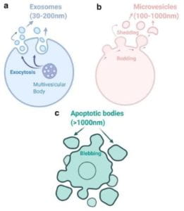
Figure 2. Descriptive images of different types of cellular vehicles

Exosomes, otherwise known as extracellular vehicles (EVs) are classified into three groups based on their size and biogenesis (footnote 7). Exosomes range from (30-200nm) to micro vesicles (100-1000) and apoptotic bodies (>1000nm) (Fig 2) (endnotes 8, 9). Exosomes are of endocytic origin (3,1), which means that they arise from the intake of material into the cell through the folding and subsequent encapsulation of the lipid membrane around the materials (Fig 1).7 EVs can be further categorized based on their density, composition, and function. EVs are membrane-bound due to their nature of being carriers of cell-cell communication. They take on a spherical shape and consist of proteins such as CD9, CD63, and CD81, which are part of the Tetraspanin family and cytoskeletal components. These vesicles, once secreted can provide key information from the cell of origin, like a “cell biopsy.”

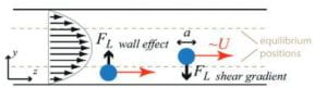
Figure 3. Effect of Channel Shape and Size on particle movement

To understand the device, the physics that drive the device must be understood. Microfluidic devices use the unique chemical and physical properties of liquids and gasses at the micro and nano scale (endnote 5). The most studied way to control the fluids is using shaped channels. Channel shapes can focus, concentrate, order, separate, transfer, and mix the particles and fluids (endnote 6). A deviation from a straight channel introduces dominant/weaker lift forces and internal lift through the interaction with the particle and the adjacent wall (Fig 3). Focusing the particles and fluid into specific shapes and channels allows the particles to self-sort and filter. Using a square channel as an example, randomly dispersed particles of a certain size will focus on four symmetric equilibrium positions near the center of the channel wall face (Fig 4 a). When an appropriate outlet design and channel shape are incorporated, then the particles can be captured with high purity, high yield, and at a high rate concerning the concentration of the solution. This allows for downstream analysis, which in this project correlates to a SERS sensor (endnote 10). The SERS sensor will be used to analyze the particles.

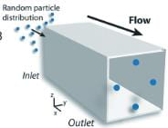
Figure 4.a. Particle orientation within a square tube on indeterminate length

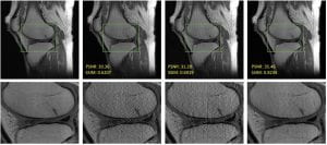
The ultimate objective of the entire apparatus is to seamlessly integrate a Surface Enhanced Raman Sensor (SERS) into the microfluidic device and enable the fluid to flow through the sensor, thus facilitating the identification of exosomes. A reservoir will hold a solution of PBS buffer and 1% Bovine, in which the exosomes will be suspended. Using a connected pump, the fluid will flow from the reservoir through the microfluidic device and get filtered before passing in front of the SERS sensor, which will help detect the exosomes. This will allow the detection of Ovarian Cancer exosomes, which can confirm or deny a diagnosis of ovarian cancer in a woman. Early diagnosis is essential for finding cancer cells. The traditional and current methods (diagnostic magnetic resonance imaging (MRI) and computed tomography (CT) are typically highly costly and come with several downsides. A high dosage of radiation in the long term can cause damage to healthy cells and may cause serious issues for the patient depending on the cells that are affected or not. The device is a rapid, non-invasive method that will allow for rapid cancer diagnosis. Notably, the device will have characteristics that improve on similar devices in the category, which are discussed in length below.

Methods/ Technical Approaches

During the initial discussions of the PDMS casting, the consensus was that different PDMS to curing agent ratios had to be synthesized to determine which ratio would yield the best overall results. Calculations were done to determine the proper breakdown of the PDMS to curing agent ratio. The initial casting dimensions were based on version 15 of the solid works models (Fig.4.b). The proper breakdown of the ratios was calculated through the simple equation of .Where the being the total internal volume of version 15 of Solid Works model. is the total number of parts. The total internal volume of version 15 of the PDMS mold was calculated to be 3.4 mL.

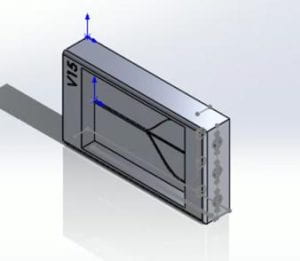
Figure 4.b. Version 15 of the microfluidic device

With the z-height being 0.5 cm, the x-height being 3.4 cm, and the y-height being 2.00 cm, resulting in a total volume of 3.4 cm3 or 3.4 mL. It was decided that the ratios that would be tested and cast would be 10:1 and 15:1. The total amounts of the required volumes for both the 10:1 and 15:1 were calculated using the equation previously mentioned. For the 10:1 and 15:1 casting, there was an assumed 0.1 mL margin of error for the castings and potential residue material that would be left behind from mixing the PDMS/Curing agent to the transfer into the models. The calculations for the 15:1 casting proceeded with a total of 16 parts being assumed, with 15 parts being PDMS and 1 part being the curing agent 3.5 mL )16=0.2187 mL 0.2187 mL∙15=3.2812 mL PDMS, 0.2187 mL curing agent. For the 10:1, the calculations were done similarly where ten parts were assumed to be the PDMS and 1 part was assumed to be the curing agent for a total of 11 parts resulting in the final equation being 3.5 mL 11=0.318 mL, 0.318∙10=3.181 mL PDMS, 0.318 mL curing.

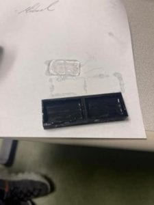
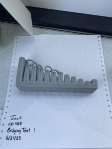
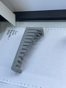
Fig. 5. The results of the casting with the 15:1 and 10:1. The initial models were cured for roughly 48 hours. Even after the 48 hours recommend curing time the PDMS molds were still incredibly unstable.

After the initial casts of the 15:1 and 10:1 mold, it was realized that the ratios of PDMS in the mixture resulted in very unstable and structurally weak molds (Fig.5). At this point in the experimental process the molds were still curing in standard room temperature, anywhere from 20-23 degrees Celsius. After it was determined that the current ratios of PDMS-to-curing agent ratios that were currently being used resulted in inadequate and unstable molds, the conclusion was made that the next sample of molds would be done in accordance with the following ratios, 11:1, 11:2, 10:1, and 10:2. Between recasting new PDMS molds the B9 printer was in need of a recalibration. Since the project was in the later stages of physical development, the decision was made that the B9 printer should be recalibrated to the desired resolution of 50 μm. The 11:1, 11:2, 10:1, and 10:2 molds were removed and examined. When the molds were released from the casts the 10:2 PDMS casts were noticeably softer and more malleable than the 11:2 casts (Fig. 6B). There also appeared to be signs of PDMS residue left behind upon removing the PDMS casting mold (Fig. 6A, D).

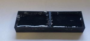
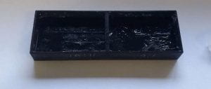
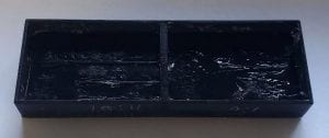
Fig 6 (A.B.C.D: top to bottom, clockwise): The results of the different PDMS curing ratios after the PDMS had been removed.

Upon the realization that the PDMS was stuck to the foundation of its mold during removal, the team made the decision to use mold release and a control group of no mold release on the casts themselves. The team made the decision that based on our previous casts we would utilize the 11:2 ratio PDMS mixture-it was the most structurally sound. On February 11th, 2023, the PDMS a new set of molds were produced 3 casts were done using mold release and 3 were done using the coconut oil. Due to the fact the oven could not be used to increase the curing time these samples were left to cure for 120 hours. Even after the 5-day curing time the molds did appear to be structurally weak (Fig.5). The way in which we have approached the current methods in casting and producing this device align with the current goals of keeping this device reusable and inexpensive.

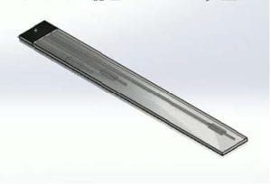
Fig. 7. Isometric view of V6 Device

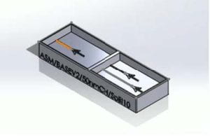
Fig. 8. Isometric View of version 11 of the device.

We have been able to create numerous models using the PDMS with little cost. We have also incorporated the technique of washing the PDMS casting trays using the chemical compound known as hexane(s) C6H14. Since hexane was utilized as a washing method-to dissolve the PDMS from the trays has allowed for the reuse of many of the casting trays and keep the costs of printing down. The cost of materials and financial use has been kept to a minimum during the project to a minimum by using low amounts of the PDMS cast silicon base and the caring agent. Based on the calculations previously mentioned, we do not use more than four grams at a time of the PDMS casting and curing agent combined. With a total of six trays for potential casts, there are no more than 24 grams used out of the 200-gram base and 20-gram curing combined.

Device Design Updates

Our previous casts we would utilize the 11:2 ratio PDMS mixture-it was the most structurally sound. On February 11th, 2023, the PDMS a new set of molds were produced 3 casts were done using mold release and 3 were done using the coconut oil. Due to the fact the oven could not be used to increase the curing time these samples were left to cure for 120 hours. Even after the 5-day curing time the molds did appear to be structurally weak (Fig.5). The way in which we have approached the current methods in casting and producing this device align with the current goals of keeping this device reusable and inexpensive.

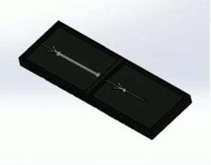
Fig. 9. Top view of version 12 of the device

We have been able to create numerous models using the PDMS with little cost. We have also incorporated the technique of washing the PDMS casting trays using the chemical compound known as hexane(s) C6H14. Since hexane was utilized as a washing method-to dissolve the PDMS from the trays has allowed for the reuse of many of the casting trays and keep the costs of printing down. The cost of materials and financial use has been kept to a minimum during the project to a minimum by using low amounts of the PDMS cast silicon base and the caring agent. Based on the calculations previously mentioned, we do not use more than four grams at a time of the PDMS casting and curing agent combined. With a total of six trays for potential casts, there are no more than 24 grams used out of the 200-gram base and 20-gram curing combined.

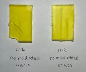
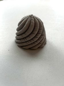
Fig 10. PDMS castings conducted on 2/16/23 where no mold release was utilized.

This section provides a detailed analysis of the advancements in device design and highlights the potential benefits and drawbacks of each advancement. Starting with Version 6 (Fig.7) the device channels and the fluid manifold were the main development. Looking at Figure 7 you can see through the translucent top piece the 3 channels sized to focus 30, 50, and 75nm exosomes. The research focus has shifted towards exploring different ratios of PDMS, in conjunction with varying mold releases and ratios. To enable this, a series of molds were developed that allowed for testing of various combinations of base-to-curing ratios, temperature, and time in the oven. To reduce material usage and accommodate size constraints, the mold size was minimized, and the channels were simplified to only 50 nm.

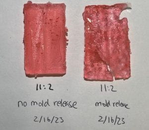
Fig. 11. Another PDMS casting that was done on 2/16/23/ Left side, was with no use of any type of pf mold release. Right side, with the use of mold release

When deciding between a negative mold (or reverse mold), which produces a negative impression of an object or pattern, and a positive mold (or direct mold), which produces a positive impression, we opted for the latter to create the microfluidic device. The process of creating a positive mold involves multiple steps, starting with mixing the base and curing agent in a specific ratio in a separate dish. The material is then poured into the mold, and air bubbles are removed either through vacuum or manually. Lastly, the mold is placed in the oven for a specific amount of time at a specific temperature.
After the mold material has hardened, it is removed from the object or pattern, revealing a positive impression of the original. The casting material fills the positive space of the mold, taking on the shape of the original object or pattern, resulting in a replica or a copy of the original. Positive molds are an efficient and cost-effective solution for creating multiple copies of an object or pattern for a wide range of applications. Versions 11 and 12 (Fig.8,9) continued the trend of incremental improvements in the mold design, while simultaneously reducing the weight of the mold itself, thus decreasing material costs. Design simplifications enabled the team to increase the effective casting area, further optimizing the device. However, during testing with thinner molds, air bubbles were observed forming on the bottom of the cast. This issue was attributed to an uneven heat distribution across the different regions of the mold. To address this problem, the team decided to keep the 5 sides of the casting mold at a uniform thickness moving forward. As previously mentioned, the ideal ratio of PDMS to curing agent was found to be 11:2, followed by a curing time of 4 hours at 50 °C, which produced the best results. Version 13 onwards, the focus shifted towards developing a functional device for testing and data analysis purposes. To achieve this objective, the team procured the GENIE Touch Syringe Pump platform from PI for precise fluid manipulation and received specialized training on the HIROX lab microscope for obtaining high-resolution images of the device during operation. While the device design is being fine-tuned and made watertight, initial observations are being carried out under a standard lab bench microscope.

Results
So far in the experimental process several microfluidic channel prototypes have been synthesized. Due to variables that have not yet been identified it has been difficult to determine what the causes of the differences of the results were. Figure 10 is an example of a cast that was conducted on February 16,2023. This PDMS was casted with no use of any type of casting mold release. Whereas in figure 11, the right-handed cast was done with the use of mold release. Through these two different samples, we concluded that the mold release in combination with the PDMS had this interaction that prevented the PDMS from fully curing. This effect is more noticeable in figure 12. On February 12, 2023, casts were also conducted. However, these results were profoundly different form the casts that were later done on the 16th. After the initial casts using the mold release, another casting was done to confirm the idea that mold release effected the structure of the PDMS (fig.11). We have however been able to determine that through our casting technique we have been able to maintain some level of resolution. Through a microscope the resolution require has been somewhat confirmed (fig.13). Even though the casting techniques have yet been perfected. The concept is there, and we have been able to produce micro channels.

Fig. 12. Two Casts that were conducted with the use of mold release.

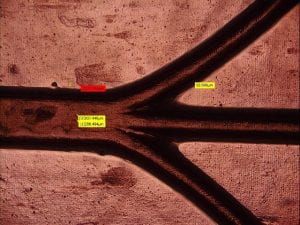
Fig. 13. HiRox microscope image of the microfluidic channels.

Endnotes

1 Siegel RL, Miller KD, Jemal A. Cancer statistics, 2019. CA: A Cancer Journal for Clinicians. 2019;69(1):7-34. doi:10.3322/caac.21551

2 Perumal J, Wang Y, Attia ABE, Dinish US, Olivo M. Towards a point-of-care SERS sensor for biomedical and agri-food analysis applications: a review of recent advancements. Nanoscale. 2021;13(2):553-580. doi:10.1039/d0nr06832b
3 Lee C, Carney R, Lam K, Chan JW. SERS analysis of selectively captured exosomes using an integrin-specific peptide ligand. Journal of Raman Spectroscopy. 2017;48(12):1771-1776. doi:10.1002/jrs.5234

4 Team E. Microfluidics: A general overview of microfluidics. Elveflow. Published online February 5, 2021. Accessed September 14, 2022. https://www.elveflow.com/microfluidic-reviews/general-microfluidics/a-general-overview-of-microfluidics/
5 Kim U, Oh B, Ahn J, Lee S, Cho Y. Inertia–Acoustophoresis Hybrid Microfluidic Device for Rapid and Efficient Cell Separation. Sensors. 2022;22(13):4709. doi:10.3390/s22134709
6 Amini H, Lee W, Carlo DD. Inertial microfluidic physics. Lab Chip. 2014;14(15):2739-2761. doi:10.1039/C4LC00128A
7 Gurung S, Perocheau D, Touramanidou L, Baruteau J. The exosome journey: from biogenesis to uptake and intracellular signalling. Cell Commun Signal. 2021;19:47. doi:10.1186/s12964-021-00730-1

8 Pegtel DM, Gould SJ. Exosomes. Annu Rev Biochem. 2019;88:487-514. doi:10.1146/annurev-biochem-013118-111902
9 Lee C, Carney R, Lam K, Chan JW. SERS analysis of selectively captured exosomes using an integrin-specific peptide ligand. Journal of Raman Spectroscopy. 2017;48(12):1771-1776. doi:10.1002/jrs.5234
10 Perumal J, Wang Y, Attia ABE, Dinish US, Olivo M. Towards a point-of-care SERS sensor for biomedical and agri-food analysis applications: a review of recent advancements. Nanoscale. 2021;13(2):553-580. doi:10.1039/d0nr06832b

Recovery of Fine Details for Fast Imaging Knee Pathologies

By Jasina Yu

Portrait of Jasina Yu

Knee diseases or injuries are very common in the United States. For example, more than 14 million Americans suffer from knee osteoarthritis. Magnetic resonance imaging (MRI), as an interdisciplinary field of computer science, mathematics, engineering, and MR physics, provides an accurate noninvasive assessment of knee pathology. The soft tissue structures (such as menisci, ligaments, and cartilage) and bone marrow of the knee can be visualized for diagnosis and prognosis. However, an MRI scan generally needs 45-90 minutes. As a freshman, I am interested in computer science, mathematics, and physics. MRI integrates those fields, and it is a great research topic to achieve my study goals.

The objective of the project is to advance our understanding of MRI by keeping fine details of knee images. Knee pathologies are accurately visualized without sacrificing imaging speed. The fundamental understanding of the feature representation, extraction, and selection in the artificial intelligence (AI)-based reconstruction process will benefit the knee pathology features’ recovery from highly undersampled data. Detailed information lost in the reconstruction process was studied. This project has helped initiate my research activities at UMD and I hope to advance my career as a researcher and innovator in biomedical imaging investigation.

Based on the preliminary research using the fastMRI dataset [1], our AI-based technique (as shown in the 4^th column of the figure above) can recover more details than the other two methods shown in the 2^nd and 3^rd columns of the figure. The reference knee image is shown in the 1^st column of the figure. Our AI method has closer pathological details to the reference knee image because the other two methods have degraded image quality.

Reference

[1]. Knoll F, et. al. fastMRI: a publicly available raw k-space and DICOM dataset of knee images for accelerated MR image reconstruction using machine learning. Radiol Artif Intell. 2020;2(1): e190007.

References

Babapour, AR., Gahassab-Mozaffari, N. & Fathnezhad-Kazemi, A. Nurses’ job stress and its impact on quality of life and caring behaviors: a cross-sectional study. BMC Nurs 21, 75 (2022). https://doi.org/10.1186/s12912-022-00852-y
Baik, S. H., Fox, R. S., Mills, S. D., Roesch, S. C., Sadler, G. R., Klonoff, E. A., & Malcarne, V. L. (2019). Reliability and validity of the Perceived Stress Scale-10 in Hispanic Americans with English or Spanish language preference. Journal of health psychology, 24(5), 628–639. https://doi.org/10.1177/1359105316684938
Centers for Disease Control and Prevention. (2022, October 14). Heart Disease Facts. Centers for Disease Control and Prevention. Retrieved December 13, 2022, from https://www.cdc.gov/heartdisease/facts.htm#:~:text=About%20697%2C000%20people%20in%20the,1%20in%20every%205%20deaths.&text=Heart%20disease%20cost%20the%20United,year%20from%202017%20to%202018.&text=This%20includes%20the%20cost%20of,lost%20productivity%20due%20to%20death.
Cohen, S., Kamarck, T., & Mermelstein, R. (1983). Perceived Stress Scale [Database record]. APA PsycTests. https://doi.org/10.1037/t02889-000
Juneau, M. (2019, May 6). Overwork can increase the risk of cardiovascular disease. Prevention Watch. Retrieved December 15, 2022, from https://observatoireprevention.org/en/2019/05/06/overwork-can-increase-the-risk-of-cardiovascular-disease/
Lee, E.-H. (2012, September 18). Review of the Psychometric Evidence of the Perceived Stress Scale. ScienceDirect. Retrieved December 14, 2022, from https://www.sciencedirect.com/science/article/pii/S1976131712000527
Saberinia, A., Abdolshahi, A., Khaleghi, S., Moradi, Y., Jafarizadeh, H., Sadeghi Moghaddam, A., Aminizadeh, M., Raei, M., Khammar, A., & Poursadeqian, M. (2020). Investigation of Relationship between Occupational Stress and Cardiovascular Risk Factors among Nurses. Iranian journal of public health, 49(10), 1954–1958. https://doi.org/10.18502/ijph.v49i10.4699
Sarafis, P., Rousaki, E., Tsounis, A. et al. The impact of occupational stress on nurses’ caring behaviors and their health related quality of life. BMC Nurs 15, 56 (2016). https://doi.org/10.1186/s12912-016-0178-y
Starc J. (2018). Stress Factors among Nurses at the Primary and Secondary Level of Public Sector Health Care: The Case of Slovenia. Open access Macedonian journal of medical sciences, 6(2), 416–422. https://doi.org/10.3889/oamjms.2018.100
Research in Computer & Information Science